Section 5
5
Measurements and Units
Measurements and Units
At the end of this lesson you should be able to:
- Define the concept of measurement.
- Name the SI standard units.
- Describe the definition of SI standard units.
- Describe the difference between accuracy and precision.
- Calculate a body density.
1.5.1 Measurements and Units
Introduction
Many properties of the universe, such as time, length, mass, etc. that are susceptible of quantifying or assigning a number are called magnitudes. The assignment usually is done with calibrated instruments. The magnitude properly quantified is called quantity..
Measurements
To quantify a physical magnitude, it is necessary to develop a procedure to assign it a number, and for this, standard units or comparison patterns are defined. The numbers assigned to a magnitude can be integers ℤ = 0, ±1, ±2, ±3⋯, or real numbers, rational like 1/3 = 0.333… or irrational like 2 = 1.41421356237309504880… (infinite numbers follow).
As stated in section 4, in the scientific method, two of the method phases require measuring. The measurement is an experimental or computational process that compares the magnitude M (measurand) of interest with the base unit [M] or dimension of the magnitude. ΙIn physics, these comparison standards or units are defined in the SI system of units. This process s of comparing produces an estimate of the true value of the magnitud, together with an estimation of the uncertainty associated with the magnitude estimate.
In the process of measuring the folloing systems may affect the results: the observer, the measuring instrument and the environment. Since not all observers, instruments an environments are equal, the result of the measurements are subject to variations from the real value of the measurand. These variations, called uncertainty δΜ = M – M, must be expressed with the best value obtained from the measurements M. The result is normally expressed in the following way:
M =
M =
For example you may say that you measured the length of a rod, and it is 15 cm plus or minus 1 cm, at a 90 percent confindence level. The result is expressed:
at 90% confidence level
Lrod = (15 ± 1) cm
(15 – 1) cm ≤ Lrod ≤ (15 + 1) cm
14 cm ≤ Lrod ≤ 16 cm .
Another way to asses the level of uncertainty in measurements is to calculate the percent of uncertainty E %, which is calculated with the formula:
T
Then the percent uncertainty is expressed as δL % = 1,5 %
How to represent the numbers that express the measurements results?
Scientific Notation
Scientific notation consists of expressing any real number as the product of a number greater than -10 and less than 10 and a power of 10. That is:
M = d∙10n ,n∊ℤ
-10 < d <10
Assuming a good knowledge of the arithmetic of numbers from 1 to 10 and a good knowledge of operations with powers, this notation helps a lot in quick calculations.
Remember that in the English language the decimal point is used as a fractional part separator: 1,200.50 means 1 thousand two hundred and fifty cents.
In many other languages (European , Russian) the decimal comma is used for fractional part separation 1.200,50 means 1 thousand two hundred and fifty cents.
To avoid confusion, scientist are strongly advised not you use periods or commas to divide groups of three digits. Instead, use a space or thin space: 1 200.
Example 1. Express in the following numbers in scientific form.
Speed of light in a vacuum: 299 792 458 ms-1 = 2.99792458 x 10⁸ ms-1.
Mass of a grape: 0.003 = 3 x 10⁻³ kg.
Example 2. Estimate the value of the expression:4238
Let’s calculate
In addition to scientific notation, it is common in the exact sciences to use prefixes to express very large or very small quantities.
In addition to scientific notation, it is common in the exact sciences to use prefixes to express very large or very small quantities. For example,
1.5 x10³ watts = 1.5 kilowatts = 1.5 kW, which is the amount of power most household appliances draw.
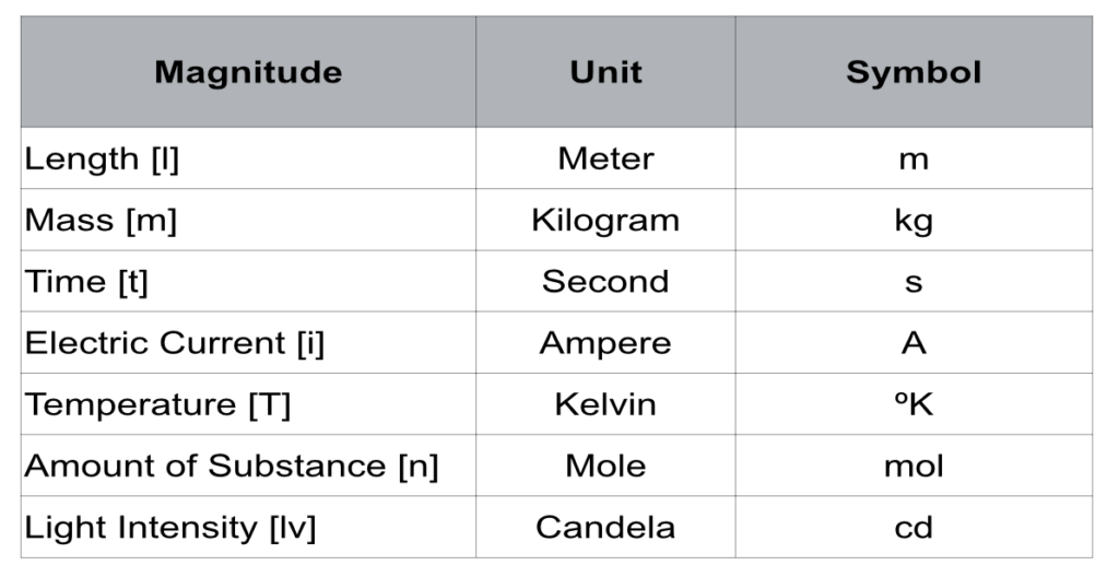
The measurement process defines an appropriate mathematical model with which the magnitudes are compared with a standard unit. If the model expires or presents problems, it should be modified. The definition of standards has evolved over time due to the variability of standards. Finally in 1791, the French Academy of Sciences created a system of units based on the invariability of standard or referent units. The system is called the International System of Units (SI) or MKSA. Currently the SI is based on seven base units that define the standards of length, mass, time, electric current, temperature, amount of substance, and light intensity (Table 1.5.1).
Standard Units of the SI System
The last revision of the International System of Units or SI was carried out on September 16, 2019. The revised SI (from French Système International d’unités) agreed on the following definitions:
Length
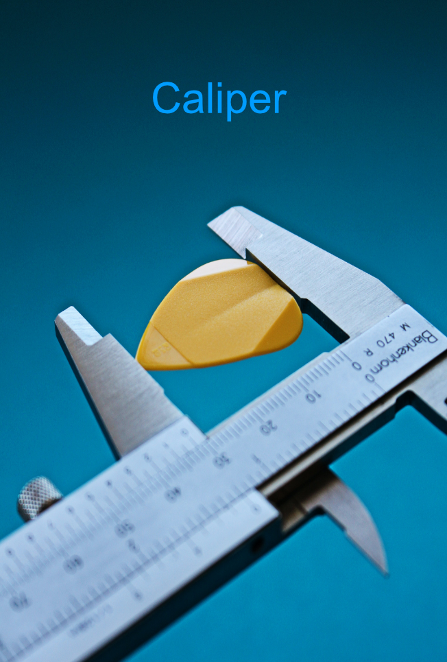
The meter, with symbol m, is the SI unit of length. A meter is the length traveled by light in a vacuum during a time interval of 1/299 792458 of a second. Lenghts are measured with rulers, vernier calipers, micrometers screw gauges, measuring tapes and odometers.
This definition solves the variability problems that the previous definition had, which defined the meter as equal to 1 650 763.73 wavelengths in the vacuum of the orange-red emission line in the electromagnetic spectrum of the krypton-86 atom.
Here the important thing to remember is that the meter is the standard unit of length and that the height of a standard table is approximately 1 m.
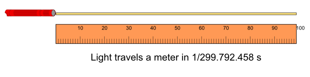
Figure 1.5.2 shows the measurement of a bar of length 1.3333 cm = 1 1/3 cm = 4/3 cm (the three with the top bar indicates that the 3 three repeats indefinitely). Here we assume that we have a ruler with 1/3 cm resolution.
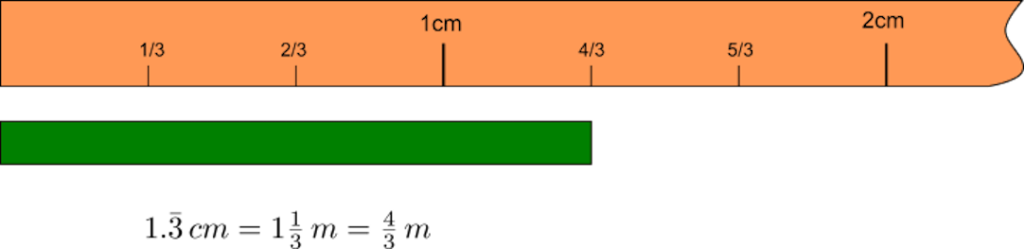
Figure 1.5.3 shows the process of measuring a rod with length 2 (if it exists as a real number!).
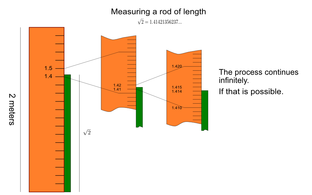
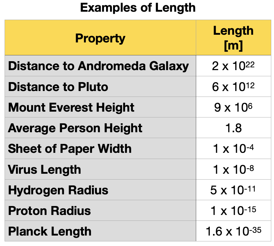
Table 1.5.2 shows some examples of the wide range of lengths observed in nature.
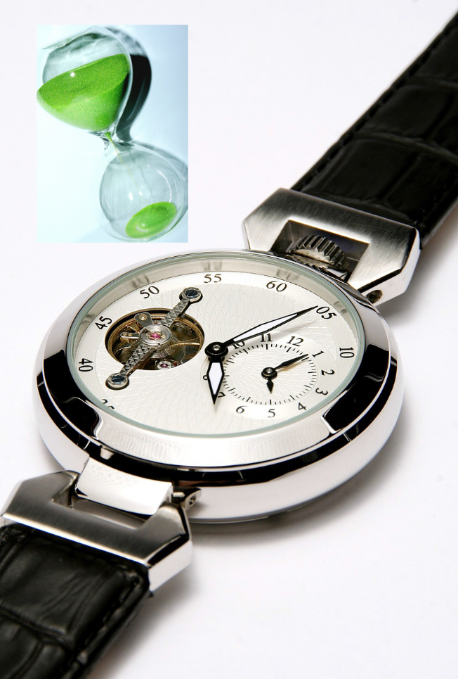
Time
The second is the SI unit of time and its symbol s. One second is the duration of 9 192 631 770 periods of the radiation corresponding to the transition between the two hyperfine levels of the unperturbed ground state of the cesium-133 atom. Time is measured with clocks and watches.
This definition solves the variability problems that the previous definition had, based on the time it takes the earth to rotate around its axis, a rotation that is slowly changing due to the interaction with the moon. The second in that definition was 1/86,400 the length of the mean solar day.
Table 1.5.3 shows examples of different orders of magnitude of electric currents observed in nature.
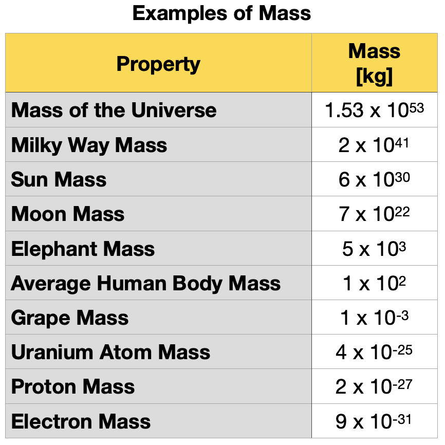
Mass
A kilogram is the SI unit of mass, and its symbol is the lowercase letters kg. Mass is measured with balances. On May 20, 2019, the kg was defined by setting the numerical value of Planck’s constant, h, as 6.62607015 x 10⁻³⁴ kg∙m2 ∙s-1, where the meter and the second are defined as a function of the speed of light in a vacuum, c and the duration of the atomic second.
This new definition is more accurate than the definition of kg given in 1899 as the mass of a right circular cylinder of height equal to that of diameter 39.17 mm made of platinum and iridium. However, this prototype was losing its mass over the years for unknown reasons.
Table 1.5.4 shows examples of different orders of magnitude of electric currents observed in nature.
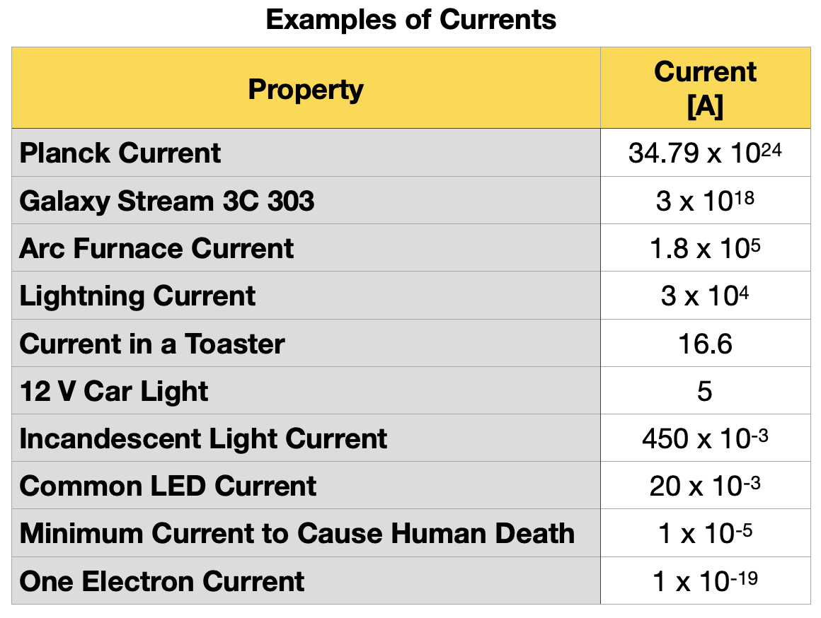
Electric Current
A kilogram is the SI unit of mass, and its symbol is the lowercase letters kg. Mass is measured with balances. On May The SI unit of electric current is the ampere, and its symbol is A. Current is measured weith ammeters. An ampere is the electric current corresponding to the flow of 6.241 509 074 x 1018 elementary charges per second. Current is measured with ammeters.
Table 1.5.5 shows examples of different orders of magnitude of electric currents observed in nature.
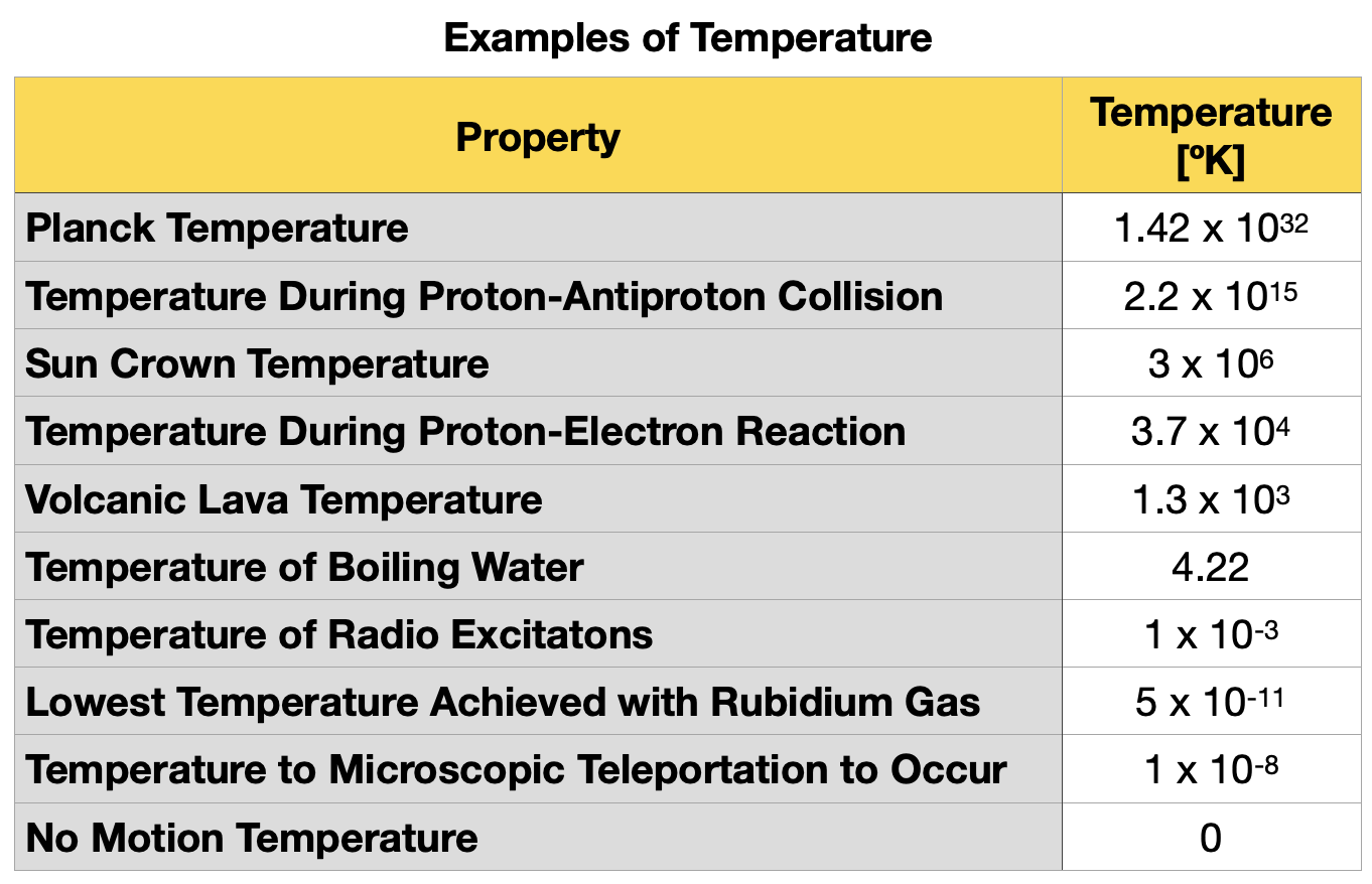
Temperature
The kelvin is the SI unit of temperature, and its symbol ºK. Temperature is measured with thermometers. One kelvin is equal to the thermodynamic temperature change that gives rise to a thermal energy change kT of 1.380 649 x 10-23 J.
Table 1.5.6 shows examples of different orders of magnitude of temperatures observed in nature.
Amount of Mass
The mole is the SI unit of quantity of substance, and symbol mole. A mole is the amount of substance in a system that contains 6.002 140 76 x 1023 specified elementary entities. Amount of subtance is measured with balances.
Light Intensity
The SI unit of light intensity is the candela, and its symbol cd. One candela is the luminous intensity, in a given direction, of a source that emits monochromatic radiation of frequency 540 x 1012 Hz and has a radiant intensity in that direction of 1/683 W/srit is measured with a photometer.
Derived Units
All other units are called derived units. Area, volume, density have derived units. The area of a parallelogram with sides l1 and l2 is given by the product A=l1x l2 m2. So m2 = m∙m square meter is the unit of area.
Another example is the metric unit of power, called a watt whose symbol is W (for Watt in English). The watt is expressed in terms of the units of mass, length and time, as will be seen later in the mechanics course,
1 W = 1kg ∙ m2/s3. which is read kilogram square meter per cubic second.
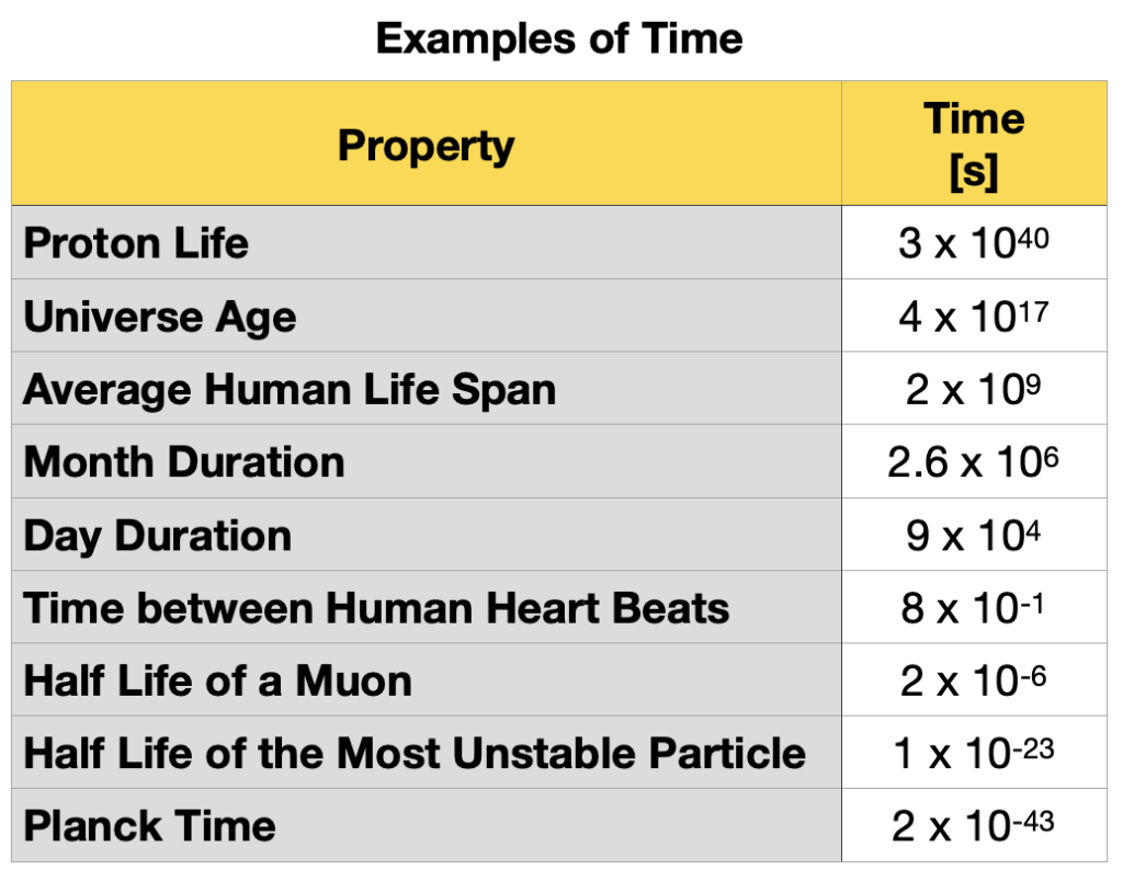
The scale of length, time and mass of matter at the atomic or subatomic level is very small compared to the scales of the same magnitudes of everyday processes. For example, the half-life of the most stable particle is of the order 10-23 s and the heartbeat time is of the order 10-6 s. The time it takes for the heart to beat once is 1017 s (317 097 919.83 centuries) longer than the particle’s half-life. For this reason, it is convenient to define multiples and submultiples of the standard units, as seen in Table 1.5.7.
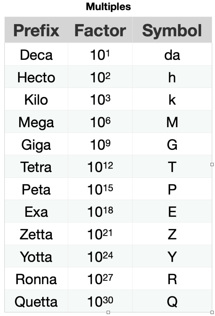
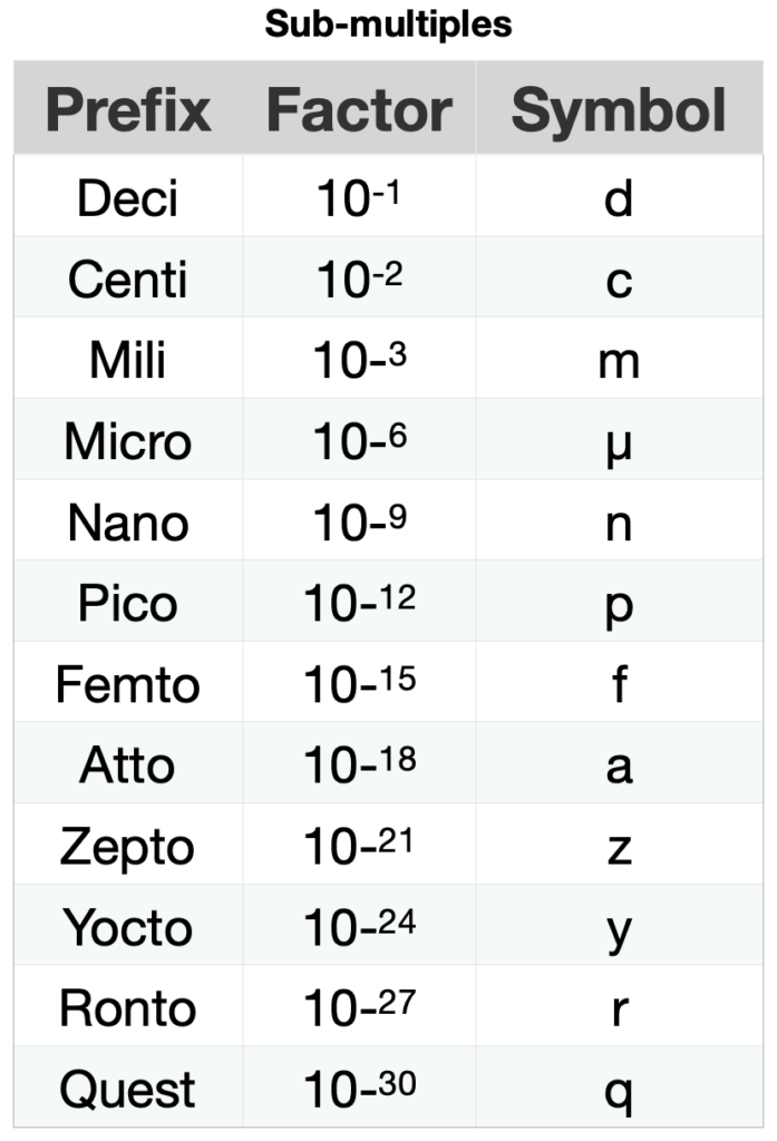
Table 1.5.7. Prefixes of the multiples and submultiples of the metric system.
Measurements Uncertainties
Uncertainties in Single Measurements
Effects of the measurement instrument
The selection of the appropriate measuring instrument is essential in the measurement process. If, for example, we are going to measure the length of a table, we can choose a ruler whose smallest divisions, called resolution, are centimeters (cm) or millimeters (mm). I think it is clear that the ruler with divisions in mm will give us better results. But if we are going to measure the thickess of a piece of paper, the ruler is naot and option, instead we may chosse a micrometer, which has much better resolution, 0.01 mm.
Well, as seen in figure 1.5.4, the right end of the table could not coincide with any cm or mm mark and consequently we would have to estimate (appreciate, guess) the fraction of centimeters or milimeters where the right side of the table ends. It is possible that the right end coincides with one of the millimeter marks and consequently give us a more precise result than the one obtained with the lower ruler. In this example, the measurement with the upper ruler is L1 = 69 mm, that means the lenght measure is closer to 69 than to 68 or 70 cm. In conclusion the best estimate is L1 = 69 mm, and the probable range 68.5 cm to 69.5 mm. The length has been measured to the nearest millimeter.

Uncertainties in Multiple Measurements
When you measure the lenght of an object, all posssible values of the length constitue a population. If you just take a few measurements, let’s say 10 measurements, then you are working with a population random sample. Suppose you measure the thicknes of the box shown in figure.
Similarly, the measurement with the lower ruler is L2 = 6.9 cm. Since the spacing is wider, you can confortably estimate where the end of the table lies. A reasonble conclusion would be L2 = 6.9 cm, and the probable range 6.8 cm to 7.0 cm. The length has been measured to the nearest millimeter.
The resolution of a measuring instrument is the smallest division of its scale. So the resolution of the upper ruler is δL1 = 0.1 cm and that of the lower one δL2 = 1 cm.
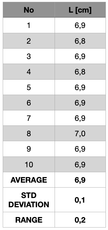
That uncertainty of a set of measurements is the range within which we believe the value of the table’s length to lie. Now, suppose ten people measure the table with the top ruler. The results in cm could be those shown in table 1.5.8. Note that the largest difference between maximum and minimum values (the range) is R1 = 7,0 cm – 6,8 cm = 0,2 cm.
If the measurements were made with the lower ruler, the results could be as shown in table 1.5.9.
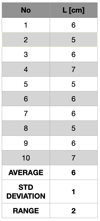
With the bottom ruler, the range of the results is R2 = 7 cm – 5 cm = 2 cm. The range gives an idea of how dispersed the results are. In this example the results obtained with the upper ruler are less dispersed and we say that they are more precise than those obtained with the lower ruler. So a set of data is precise, repeatable and reproducible if the data are close to each other, compared to another set of data from the same measurement. One common way to estimate the measurement uncertainty is to accept half of the range. So in the case of the measurements performed with the upper ruler the range estimated uncertainty would be R1/2 = 0,1 cm, and for the measurements with the lower ruler R1/2 = 1 cm.

The accuracy of the data is related to the average value of the acquired data. The closer the data is to the real value (mean value), the more accurate it will be.
In the table example, the average value of the data obtained with the upper ruler is 6.9 cm.
Note that the farthest value is 7.0 cm and its distance from the mean value is 0.1 cm.
With the lower ruler the average value is 6 cm.
In this case, the furthest value is 5 cm or 7 cm, and its distance from the mean value is 1 cm. Consequently, the data obtained with the upper ruler are more accurate than those obtained with the lower ruler, since its distance from the supposed real value (the average value) is smaller.
There are several ways to estimate the measurements uncertainty, depending on the situation:
- Use the instrument resolution, 1 mm. Then the result is expressed as L = (69 ± 1) mm
- 2. Beginner’s Guide to Uncertainty of Measurement (Bell, 1999), which is freely available on the World Wide Web.
- Use the measurements standard deviation 1 mm. Then the result is expressed as L = (69 ± 1) mm.
Percent of Uncertainty
Another way to asses the level of uncertainty in measurements is to calculate the percent of uncertainty E %, which is calculated with the formula:
Then the percent uncertainty is expressed as δL % = 1,5 %
Significant figures of a measurement
In order to explain the concept of significant figures of a measurement, let’s consider the following experiment. We want to determine the length of a green bar. For this, we are going to use a ruler with 1 millimeter (mm) resolution.
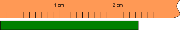
As seen in Figure 1.5.5, the length of the green bar is between 23 and 24 mm, but we don’t know exactly if it is 23,4 or 23,5 mm. A good visual estimate would be 23,5, but 5 is uncertain. There is absolute certainty about digits 2 and 3. The digits about which there is absolute certainty plus the first estimate are called significant figures.
Bibliography
- Taylor, John. Introduction to error analysis, the study of uncertainties in physical measurements. University Science Books, New York, 1997.
- Beginner’s Guide to Uncertainty of Measurement (Bell, 1999), which is freely available on the World Wide Web.